Bring Your Tiller Transactions Sheet to Life with Conditional Formatting

I started using Tiller in October of 2020 after using Mint for many years, and Quicken before that. 

Those tools imported transaction information just fine, but once I had the transactions, what I could do with them was limited to the tools the programmers provided.  When I found Tiller, the thing I immediately loved was the ability to customize.

One of the early customizations I applied to my Foundation Template was something from a post in the Show & Tell section of the Tiller Community called Custom Formatting for Your Sheets (shout out to @juno!). 

The post demonstrated how you could use a Google Sheets feature called Conditional Formatting. 

Using this feature, you could make the formatting of your cells, rows, and columns look different based on the criteria that you determine.  This seemed like the perfect way to make the Transactions sheet easier to understand.  

As an example, here’s a section of data from a Tiller Transactions sheet.  Lots of information, but hard to read:

Making sense of this requires some focus since it all just blends together. 

What if we could make it more readable? 

When dealing with transactions like this, I found a great way of doing that is to make it obvious which transactions are ‘Income’, and which are ‘Expenses’.  (Note that the following is based on Google Sheets, but Excel has the same feature, and it works in a very similar way.)

Here’s how I use Conditional Formatting to make my Income and Expenses transactions stand out:

1. While you are in the Transactions sheet, go to the Format menu and choose Conditional formatting.
2. A sidebar will open and will start a new rule for you to configure.
3. In the field below Apply to range enter A2: followed by the letter of the last (right-most) column with data in your Transactions sheet. I entered A2:W in mine. This is the range that we want to apply the formatting to.
4. In the field below Format cells if… click the dropdown and choose Custom formula is.
5. In the field that says Value or formula enter =$E2>0. This sets the condition to look in column E (that’s where my Amount column is, change the letter if your Amount is in a different column) for any amounts that are greater than 0.
6. In the Formatting style area, choose the formatting that you want to apply to any rows where the Amount is greater than 0. You can apply Bold, Italic, Underline, Strikethrough, Text Color and Fill Color. In my case, I set the Text Color to dark green 2 (click on the Text Color button and hover over any color to see the name of the color) and the Fill Color to light green 3.
7. Click Done and any transactions with an Amount larger than 0 should get the formatting you chose.
8. Click + Add another rule in the Conditional format rules sidebar and repeat the same process, but for the second rule the custom formula will be =$E2<0, and the formatting I applied was Text Color to dark red 1 and Fill Color to light red 3.
9. Click Done and any transactions with an Amount less than 0 should get the formatting you chose.

This is much nicer to look at!  You now get a quick feel for where you made money and where you lost money without having to read.

This not only makes it easier to locate a transaction you’re looking for, but the colored rows make it easier to read from left to right through the transaction.

To take it a step further, we can add some more useful information through formatting. 

Transfer transactions aren’t truly income or expenses, so I’d like to make them look less important.

1. Using the same process as above, create a new rule (+ Add another rule) with the same range.
2. For the custom formula, I set mine to =$D2=”Transfer” which tells it to look in column D (where my Category is) for Transfer.
3. Set your formatting options (I set the Text Color to dark gray 4 and the Fill Color to light gray 1) and click Done.

If your transaction sheet didn’t gain any new formatting, it’s likely because Conditional Formatting rules are followed in a specific order, and once a rule is met, no more rules are considered. 

In our case, because we created the ‘amount’ rules first, they will be met before it considers the ‘transfer’ rule (unless you have a transaction for $0 which won’t meet either of the two ‘amount’ rules we created.  

To fix this, in the Conditional format rules sidebar, move your cursor over the ‘transfer’ rule that you just created, and notice three vertical dots appear on the left edge of the rule. 

Move your cursor over those dots and it will turn to a four-way arrow.  Click and drag that rule up the list till it is above the other two rules and let go.  You have now set that rule to be considered first, and you should immediately see it apply to your Transactions sheet.

Now you can see Income, Expenses, and Transfers!

Here’s one more example of how I use formatting to make my Transactions sheet easier to read and more informative. 

I like to have my attention drawn to the larger transactions since they are more likely to affect my budgeting.  To do this, I set rules to make the text for large transactions bolder.

1. Click on the ‘green’ rule (amounts greater than 0) you created in the Conditional format rules sidebar, and it will go into ‘edit mode’ where you can edit the rule’s settings.
2. At the bottom of the rule, click + Add another rule.  This will create a new rule with the same settings as the last rule, making it easier for us to just change a couple things.
3. Change the custom formula from =$E2>0 to =$E2>100
4. In the formatting options, change how you’d like these larger amounts to be shown.  In my case, I changed the Text Color to dark green 3, and I turned on Bold.
5. Click Done and you’ll see the new rule added to the list below the one you originally selected.  The problem is the rule for any Amount greater than 0 will be met before there is a chance to evaluate the new Amount greater than 100 rule.  The fix is to drag the new rule higher in the list so it is evaluated first, so large amounts become bolded, then smaller amounts will be caught by the next rule.
6. Do the same thing for the ‘red’ rule (amounts less than 0), changing the custom formula from =$E2<0 to =$E2<-100, and selecting the format changes you’d like to see (I set Text Color to dark red 2 and turned on Bold).
7. Click Done and admire your work…

That’s a lot different from the first illustration of our plain transactions sheet.  We can easily see income vs expenses vs transfers and can distinguish the larger transactions from the smaller ones all at a glance. 

If you followed along, your Conditional format rules sidebar should look something like this:

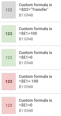
The beauty is you can fully customize this any way you like. 

If you want different colors, you can choose from the list they provide, or even input a custom color, making your choices almost endless.  You don’t think $100 is a large transaction?  Fine!  Choose any number you like! 

There are other ways this can be used as well.  I have a workflow to reconcile my Transfer transactions, and use conditional formatting to change any transactions to Orange that have a category of Transfer In or Transfer Out, but don’t have a Tag that contains Match, so I know they need attention. 

The options are only limited to your imagination (and your ability to figure out a formula to make it work)!  Oh, keep in mind that you can use Conditional Formatting on ANY of your sheets!

If you have ideas for ways to use Conditional Formatting on your template but aren’t sure how to make it work, post a question in the Tiller Community, there are lots of people like myself that are willing to help.  The great thing about posting your question is that others may realize that they could benefit from what you’re trying to do, and once we come up with a solution, we all benefit!

Visit Joseph Fieber’s website at JosephFieber.com