Budgeting With Google Sheets: 18 Simple, Effective Tips

Many of us sat through countless high school classes on how to use Excel.
Those classes served us well. We can effectively budget, analyze data for work and create beautiful charts with just a few clicks of a button.
But since we’ve come of age, there’s a new player in the market: Google Sheets—the platform Tiller uses to help you build a budget, track spending, and understand your money.
Budgeting With Google Sheets
In this age of chatbots and AI, it may seem old-fashioned or unsophisticated to budget in a spreadsheet. However, the biggest companies in the world run on spreadsheets. And in a national survey, Tiller found 96% of people who track their finances are satisfied with using a spreadsheet compared with an app.
Likewise, 92% are more aware of their spending habits when they use a spreadsheet compared to an app or service.
In the spreadsheet arena, Google Sheets is rapidly catching up with Excel for personal use.
A recent survey by Tiller Money found that when it comes to using a spreadsheet for personal finance, Google Sheets is as popular as Excel for people aged 18-24.

Budgeting with Google Sheets offers many of the same workflows and benefits as budgeting with Excel.
However, Google Sheets has some not-so-obvious tricks and features that you’ll want to know.
Here are 18 simple tips on more effective budgeting with Google Sheets.
- Budgeting With Google Sheets
- 1. Use a Google Sheet Template
- 2. Send an Email for Joint Budgeting
- 3. Add Emotions to Your Money
- 4. Protect Data in Specific Cells
- 5. Use Keyboard Shortcuts
- 6. Use a Heat Map to See Your Biggest Spending Areas
- 7. Use SQL to Find Big Debits
- 8. Import Data from Other Sheets
- 9. Predict Future Income or Spending with the Growth Function
- 10. Look at Your Version History to See Past Edits
- 11. Translate a Language
- 12. Add Different Currencies
- 13. Filter Your Expenses by Category
- 14. Use the Trim Function to Get Rid of Weird White Space
- 15. Use the Proper Function to Fix Capitalization
- 16. See How Much Money You Spent at a Specific Store
- 17. Pull Stock Prices Using Google Finance
- 18. Download For Use Offline
1. Use a Google Sheet Template

Google Sheets has tons of budgeting templates you can use. This one took me about two seconds to pull up. On top of built-in categories and formulas to track expenses and income, it comes with pre-formulated charts and graphs to help you visualize your personal finances with minimum Sheets skills required.
(Click to see a list of premium Tiller-powered Google Sheets templates.)
2. Send an Email for Joint Budgeting

Let’s say you’re working together with your partner on your finances. You’re tracking expenses and transactions, when all of a sudden you come across a $300 Amazon charge in the “Entertainment” category. You can easily comment, using the @ symbol before an email address, to send an email with your inquiry directly to your partner in real time.
This is how you find out your family now owns an Xbox, and opens up a big conversation about the need to communicate before spending large sums of money.
That’s not experience talking or anything…
(Read “How to Send an Automatic Email Reminder from a Google Spreadsheet“)
3. Add Emotions to Your Money

Maybe you’re not thrilled about that Xbox purchase. You can express your displeasure in Google Sheets by using the =char() function.
First, go to Graphemica. Then, search for the fun (or angry) character you’d like to include in Sheets. Once you find it, look for the number portion of the HTML Decimal Entity. Then, simply put this number in between the parentheses in your formula.
For example, the function to insert the angry face is =char(128554).
The function to insert the house icon is =char(127960).
And so on. You can use these characters to express joy when you stay within your budget for a specific category, or disappointment when you go over. The more happy faces you have, the better.
4. Protect Data in Specific Cells

Maybe your partner thinks it’s funny to change that angry icon into a video game controller icon. But you don’t.
You can lock the data in a cell or a range of cells by highlighting it, and then right-clicking. Scroll down until you get to the “Protect range…” option. Click on it, and you’ll then be able to restrict who can edit the data in that specific cell.
5. Use Keyboard Shortcuts

We’re all familiar with “Ctrl+C” and “Ctrl+V” for copy and paste. But there are a ton of other keyboard shortcuts you can use, and Google Sheets is happy to teach you them all.
To learn how to fill ranges, insert specific functions, move between sheets and more, simply click on “Help” in the toolbar, and then click on “Keyboard shortcuts.”
6. Use a Heat Map to See Your Biggest Spending Areas

Visual learner? A heat map may just be your best friend. It allows you to see the top areas your money is going and then decide if those areas the most important to you in terms of personal values. If they’re not, you know you need to adjust your spending next month.
To do this, highlight your numbers and right click. Choose “Conditional formatting”, and then use the menu that pops up on the right-hand side of your screen to apply the heat map.
In this example, the largest spending area is housing. Following that top category are insurance, transport, groceries and setting some aside for savings.
(Read “How to Track Daily Average Spending Trends in Google Sheets“)
7. Use SQL to Find Big Debits

SQL is essentially like writing code. We’re going to make it easy for you, though, so you can use it to identify large or small charges. This can help you identify fraud, stare your biggest spending sprees straight in the face or rethink how quickly your Starbucks habit adds up.
The first thing you’re going to want to do is highlight all of your data. From there, right click and select, “Named ranges…”
In the first box, name the data. We named this dataset “March18Expenses”. You’re going to use this name to write a query.
The next thing we did was hop over to box F1, which is where we wanted to arrange our data a little differently. In that box, we wrote the following function:
=QUERY(March18Expenses, “SELECT A, D WHERE D > 100”,1)
This query pulls the data from columns A and D, but only when D is greater than $100. If you wanted to do small purchases, you could do the same thing except you’d type something along these lines:
=QUERY(March18Expenses, “SELECT A, D WHERE D < 10”,1)
8. Import Data from Other Sheets

Let’s say you have multiple files going. One is for your expenses for the entire year, and one is for your expenses, income, and investments for March of 2018. You can import your March expense data from the original file.
To do this, you are going to fill in the blanks of this code in the new file, in A1 of the “Expense” tab:
=IMPORTRANGE(“URL”,”TAB NAME!FIRST CELL IN RANGE:LAST CELL IN RANGE”)
First, grab the sharing link for your original file. You’re going to insert that where it says “URL”. In the end, our function ended up looking like this:
=IMPORTRANGE(“https://docs.google.com/spreadsheets/d/1MlNGnXAVmG95adWugFPgWSnzBQhHUz4TT7mA-YTSEHI/edit?usp=sharing”,”March 2018!A1:D19″)
The cool thing about this feature is that if I edit any information in the “Expenses” file, it will automatically update in the “March” file. That means you only have to update your numbers once rather than going through the tedium of updating them in each and every file where you have inserted the data set.
9. Predict Future Income or Spending with the Growth Function

Google sheets has a growth function which allows you to predict future expenses based on past spending patterns. This could also work with income—whether you receive a steady paycheck or are a freelancer.
You’ll need at least three data points for this to work effectively. For this chart, we used spending by category from March through May to predict spending across categories for the months of June through August. To do that, we used this function:
=GROWTH(FIRST CELL IN RANGE:LAST CELL IN RANGE)
In the image above, you can see that for Utilities, we used the specific function:
=GROWTH(G10:I10)
Pretty cool, right?
It’s important to factor in variables when you do this, though. While the grocery predictions may be relatively accurate, your utilities are likely to go up over the summer if you live somewhere hot and have AC. Be sure to be smart about your predictions, and don’t rely entirely on this function.
10. Look at Your Version History to See Past Edits

If you’re unhappy with the way your partner has edited your sheet, or you just get frustrated and give up on a new equation, you can easily look at past versions of your sheet—and restore it! Just go to “File” and then select “Version history”. The final step is to click “See version history”.
11. Translate a Language

You took a trip abroad, and when your checking account statement came in, there were all kinds of crazy characters you didn’t know how to read. You don’t know what the charge is for—even after importing your statement via Tiller.
This is where the GOOGLELTRANSLATE function comes in. The code is going to look like this:
=GOOGLETRANSLATE(“text you want to translate”, “two letter code for source language”, “two letter code for target language”)
In our example, you know you headed to Japan at the end of April, so you’re confident the source language is Japanese. Your function looks like this:
=GOOGLETRANSLATE(“ペンギンのいる”, “JA”, “EN”)
Google tells you the text means, “It is the penguin”.
Yeah, it’s not a perfect system, but it’s enough of a hint to let you know this charge is from the Penguin Bar in Tokyo.
12. Add Different Currencies

If you for some reason need to note the transaction in its native denomination, you can format cells to a certain currency by clicking on:
Format→Number→More Formats→More currencies…
13. Filter Your Expenses by Category

To filter your expenses by category, highlight your category column. Then, hit the filter button. From there, click the icon with three lines in A1. Deselect all the categories you do not want included. For this example, we filtered out all expenses except Dining Out. Click “OK” and only your Dining Out expenses will show up!
14. Use the Trim Function to Get Rid of Weird White Space

Let’s say that when you imported your transaction data from your bank, the formatting got all funky. There are a couple functions you can use to change this. The first one is trim. This function is best to use if there’s too many spaces before or between words. Here is the function you should use:
=TRIM(CELL NUMBER HERE)
15. Use the Proper Function to Fix Capitalization

If capitalization got screwy when you imported, you can fix it by using the proper function:
=PROPER(CELL NUMBER HERE)
16. See How Much Money You Spent at a Specific Store

Want to see how much money you spent at a specific store this month? Then you’ll want to familiarize yourself with the SUMIF function. First, you want to type the name of the store in a cell—you will find this in G1 in our example.
Then, you’ll want to identify the range of the column you want to search for store names. In our case, that’s A2:A20.
Finally, identify the range of the debits you want to search for spending. Above, that’s going to be D2:D20.
You’ll plug all of that into a function that looks like this:
=SUMIF(A2:A20, G1, D2:D20)
Then you’ll get your answer. You spent $125.25 at Cogos this month—gas isn’t cheap!
17. Pull Stock Prices Using Google Finance

If you’re trying to track your investments, one way to do that is through the Google Finance function. All you have to do to get live pricing is use the following function:
=GOOGLEFINANCE(“YOUR INVESTMENT’S TICKER”)
For example, above you can see the formula for Tesla as:
=GOOGLEFINANCE(“TSLA”)
18. Download For Use Offline

Want to edit your sheet while you’re on the plane, but don’t necessarily want to pay for in-air WiFi? You can easily download your work for later use offline. The above image shows the path you’ll use to get an Excel document.
Bonus: Get Tiller Money!
You can use any of these tips within Tiller’s system or without. But if you’re feeling more overwhelmed than excited after reading this article, using a service like Tiller is a great way to get your budgeting done beautifully—without needing a cheat sheet for the functions and keyboard shortcuts.