How To Easily Create A Google Sheets Pivot Table

A Google Sheets pivot table is one of the most powerful tools for understanding complex data, including your spending and personal finances. Even better, pivot tables are easy to use.

What is a pivot table?

A pivot table is a type of chart that groups and summarizes data to provide insights into trends, patterns, and outliers. They are an invaluable tool for understanding numbers.

In Google Sheets, creating a pivot table is easy and straightforward, allowing you to summarize your data with just a few clicks.

They’re also highly customizable, letting you filter and arrange your data in unique and visual ways. Whether you’re new to Google Sheets or an experienced user, learning how to use pivot tables is a must.

Tips for getting started with your Google Sheets pivot table

If you want to use Pivot Tables in Google Sheets effectively, start by organizing your data set. Make sure each column has a header.

It’s also helpful to understand the three key components of a pivot table:

• Rows represent categories or groups that aid in analysis
• Columns break down data into subcategories for better understanding
• Values indicate the summarized data like counts or sums.

Explore the main features of the Pivot Table editor, including the grouping, filtering, and sorting functions.

Finally, make sure to refresh your data source regularly so changes are reflected in your pivot table. (If you’re tracking your budget in Google Sheets, Tiller will keep your daily finances updated automatically.)

Here’s a quick video showing how to make a pivot table that clarifies spending trends:

How to create a pivot table in Google Sheets

1 – Open your spreadsheet. Select all data you want to analyze in a pivot table.

2 – With your data selected, click Insert > Pivot table in the top menu.

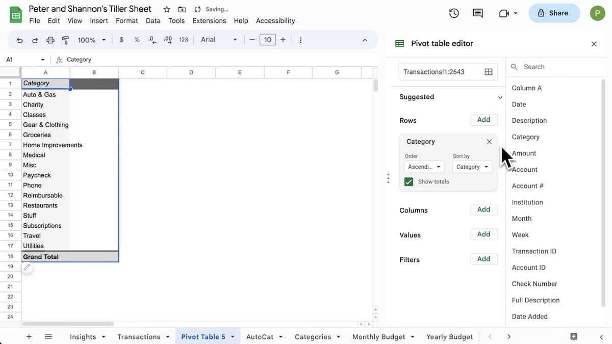
3 – A new pivot table sheet will appear with a pivot table editor panel on the right side of your screen.

4 – In the Pivot table editor panel, next to “Rows” or “Columns,” click Add, then choose the value you want to display in rows, columns, and values.

Note: Sometimes, you’ll see recommended pivot tables based on the data you choose. To add a pivot table, under “Suggested,” choose a pivot table. To turn these suggestions off, click Tools > Autocomplete then turn off Enable Pivot table suggestions.

5 – View your Google Sheet pivot table.

6 – Explore different ways of summarizing your data using Pivot Table Suggestions or the Explore Tool without worrying about manual errors. For example, you can format headers or use Slicer Dropdown before pivoting back to your original dataset.

Sorting and filtering your data

Sorting and filtering your data in Google Sheets pivot tables is an essential step for analyzing and organizing your data.

Sort your data

To sort your data, simply click on any cell in the column you want to sort by and then click on either ‘ascending’ or ‘descending’ depending on how you want to organize the data.

via Google: You can change how your data is listed, sorted, summarized, or filtered.

Filter your data

To better analyze specific data subsets while working with pivot tables in Google Sheets, use filters. They allow you to focus on particular categories or values within your data set.

Adding filters is easy:

• Select a range of cells, then click Data > Create a filter, or 
• Right-click on a cell or a range of cells, then click Create a filter

Next, choose your filter options:

• Go to the top of the range and click Filter 
• Filter by condition: Choose conditions or write your own.
• Filter by values: Hide data by unchecking the data point and click OK.
• To create a filter by cell value, right click on a cell then click Filter by cell value.
• Search: Search for data points by typing in the search box.
• Filter by color: Choose which text or fill color to filter by. You can filter by conditional formatting colors, but not alternating colors.

To remove the filter, select an option:

• Click Data > Remove filter.
• Right click on any cell then click Remove filter.

Note: When you add a filter, anyone with access to your spreadsheet will see the filter too. Anyone with permission to edit your spreadsheet will be able to change the filter.

Additional Google Sheets pivot table tips and tricks

Using multiple value fields

This feature enables you to compare and analyze different aspects of your data set quickly from different perspectives. Adding multiple values fields is easy; just drag and drop them into the “Values” section of the pivot table editor. Customize each calculation type (sum, count or average). Label each value field clearly so that you can easily interpret your results.

Changing aggregation types

In a Google Sheets pivot table, changing aggregation types is essential to summarizing your data effectively. You have several options available, such as sum, count, average, and more. To change the aggregation type for a specific field, simply click on the dropdown arrow next to the field name in the pivot table editor. This will help you better analyze your dataset and make more informed decisions based on your underlying data. Keep experimenting with different ways of using pivot tables and exploring the tool to take your analysis to the next level.

Use Charts and Slicers

Finally, add charts like Pivot Charts or Slicers to make visualizing data much easier.

The pivot possibilities are endless

Pivot tables allow you to slice and dice your financial transaction data any way you like. A table that shows spending allows you to broaden the focus of your money management. If we monitor how much we spend on eating at restaurants our monthly pivot table shows us the general trend around that spending over several months.